In a recent post I introduced three existing approaches to explain individual predictions of any machine learning model. After the post focused on LIME, now it’s the turn of IME (Interactions-based Method for Explanation), a method presented by Erik Strumbelj and Igor Kononenko in 2010. Recently, this method has also been called Shapley Values.
Intuition behind IME
When a model gives a prediction for an observation, all features do not play the same role: some of them may have a lot of influence on the model’s prediction, while others may be irrelevant. Consequently, one may think that the effect of each feature can be measured by checking what the prediction would have been if that feature was absent; the bigger the change in the model’s output, the more important should be the feature.
However, observing only a single feature at a time implies that dependencies between features are not taken into account, which could produce inaccurate and misleading explanations of the model’s decision-making process. Therefore, to avoid missing any interaction between features, we should observe how the prediction changes for each possible subset of features and then combine these changes to form a unique contribution for each feature value.
Precisely, IME is based on the idea that the feature values of an instance work together to cause a change in the model’s prediction with respect to the model’s expected output, and it divides this total change in prediction among the features in a way that is “fair” to their contributions across all possible subsets of features.
Basics of Cooperative game theory
A cooperative (or coalitional) game is a tuple ({1,…,p},v), where {1,…,p} is a finite set of p players and v: 2ᵖ → ℝ is a characteristic function such that v(∅)=0.
Subsets of players S⊂{1,…,p} are coalitions and the set of all players {1,…,p} is called the grand coalition. The characteristic function v describes the worth of each coalition. We usually assume that the grand coalition forms and the goal is to split its worth (defined by the characteristic function) among the players in a “fair” way. Therefore, the solution is an operator φ which assigns to the game ({1,…,p},v) a vector of payoffs φ=(φ₁,φ₂,…,φₚ).
For each game with at least one player there are infinite solutions, some of which are more “fair” than others. The following four properties are attempts at axiomatizing the notion of “fairness” of a solution φ:
Axiom 1: Efficiency
φ₁(v)+φ₂(v)+…+φₚ(v) = v({1,…,p})
Axiom 2: Symmetry
If for two players i and j, v(S∪ {i})=v(S∪ {j}) holds for every S, where S⊂ {1,…,p} and i,j∉ S, then φᵢ(v)=φⱼ(v).
Axiom 3: Dummy
If v(S∪{i})=v(S) holds for every S, where S⊂ {1,…,p} and i∉ S, then φᵢ(v)=0.
Axiom 4: Additivity
For any pair of games v, w:φ(v+w)=φ(v)+φ(w), where (v+w)(S)=v(S)+w(S) for all S.
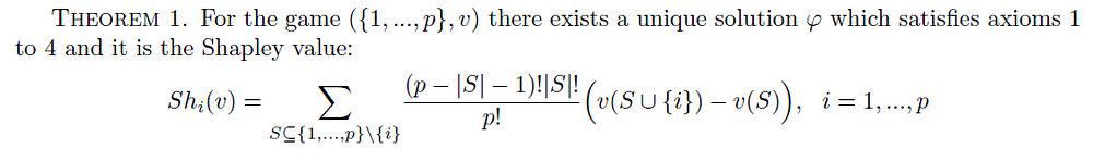
The Shapley value is a “fair” way to distribute the total gains v({1,…,p}) to the p players in the sense that it is the only distribution with the four previous desirable properties.
Moreover, there is an equivalent formula for the Shapley value:
where Sₚ is the symmetric group of the finite set {1,…,p} (i.e., the set of all permutations of the set of players {1,…,p}) and Pre^i(O) is the set of players which are predecessors of player i in permutation O∈ Sₚ (that is, the numbers that appear before number i in permutation O∈ Sₚ).
Method
Let X = X₁× X₂×…× Xₚ be the feature space of p features, represented with the set {1,…,p}.
Let f be the model being explained. In classification, f(x) is the probability (or a binary indicator) that x belongs to a certain class. For multiple classes, IME explains each class separately, thus f(x) is the prediction of the relevant class. In regression, f(x) is the regression function.
Finally, let y=(y₁,…,yₚ)∈X the instance from the feature space whose prediction we want to explain.
Strumbelj and Kononenko define the prediction difference of a subset of feature values in a particular instance as the change in expectation caused by observing those feature values. Formally:
Let f be a model. Let S={i₁,i₂,…,iₛ}⊆{1,…,p} be a subset of features. The prediction difference Δʸ(S) of the subset of features S⊆{1,…,p} in instance y=(y₁,…,yₚ)∈X is:
Note that Δʸ defines a function Δʸ: 2ᵖ → ℝ from the set of all possible subsets of features to ℝ that satisfies Δʸ(∅)=E[f(X₁,…,Xₚ)]-E[f(X₁,…,Xₚ)]=0. Therefore, Δʸ is a valid characteristic function for the cooperative game with the p features as players. Therefore, ({1,…,p}, Δʸ) forms a cooperative game as defined before. In other words, IME considers features to be players of a game where the worth of the coalitions is the change in the model’s prediction defined by Δʸ, so the goal of IME is to split the total difference in prediction Δʸ({1,…,p}) among the features in a “fair” way.
The suggested contribution of the i-th feature for the explanation of the prediction of y is the Shapley value of the cooperative game ({1,…,p}, Δʸ):
Let {1,…,p} be the set of features and let Δʸ be the prediction difference defined as above. The contribution of the i-th feature for the explanation of the prediction of y is:
Or, equivalently, using the alternative formula for the Shapley value:
where Sₚ is the set of all permutations of the set of features {1,…,p} and Pre^i(O) is the set of features which are predecessors of feature i in permutation O∈ Sₚ.
Note that this definition of contributions is not casual: the Shapley value $φ$ of a coalitional game ({1,…,p},v) is a “fair” way to distribute the total gains to the p players. In our case, axioms 1 to 3 become three desirable properties of IME as an explanation method:
That is, the sum of all p contributions in an observation’s explanation is equal to the difference between the model’s prediction for the instance and the model’s expected output given no information about the instance’s feature values. This property makes contributions easier to compare across different observations and different models.
2. Symmetry axiom:
If for two players i and j, Δʸ(S∪ {i})=Δʸ(S∪ {j}) holds for every S, where S⊂ {1,…,p} and i,j∉ S, then φᵢ(Δʸ)=φⱼ(Δʸ).
In other words, if two features have an identical influence on the prediction, they are assigned identical contributions.
3. Dummy axiom:
If Δʸ(S∪{i})=Δʸ(S) holds for every S, where S⊂ {1,…,p} and i∉ S, then φᵢ(Δʸ)=0.
That is to say, a feature is assigned a contribution of 0 if it has no influence on the prediction.
Both the magnitude and the sign of the contributions are important. First, if a feature has a larger contribution than another, it has a larger influence on the model’s prediction for the observation of interest. Second, the sign of the contribution indicates whether the feature contributes towards increasing (if positive) or decreasing (if negative) the model’s output. Finally, the generated contributions sum up to the difference between the model’s output prediction and the model’s expected output given no information about the values of the features. In summary, we can discern how much the model’s output changes due to the specific feature values for the observation, which features are responsible for this change, and the magnitude of influence of each feature.
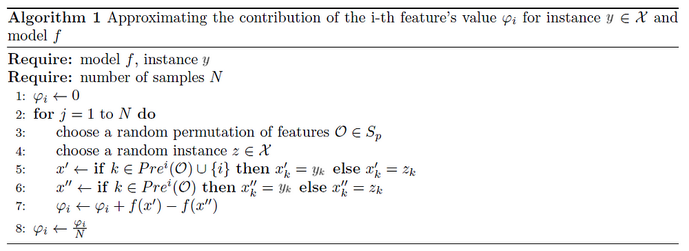
In practice, the main challenge of this method is the exponential time complexity because the computation of the contributions requires to use all possible subsets of features. To avoid this issue, Strumbelj and Kononenko developed an efficient sampling procedure to approximate feature contributions by perturbing the instance’s input features:
Note that f(x’) and f(x’’) are the classifier’s predictions for two observations, which only differ in the value of the i-th feature. They are constructed by taking instance z and then changing the value of each feature which appears before the i-th feature in order O (for x’, the i-th feature is also changed) to that feature’s value in the observation we want to explain y.
Example
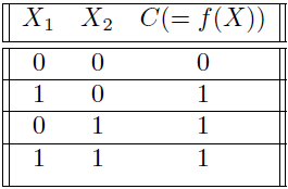
Let X₁, X₂ be two binary features, C={0,1} a binary class, and X={0,1}×{0,1} our feature space. We assume that all feature value combinations are equiprobable, as seen in the table below.
Assume that the class is defined by the disjunction C=X₁∨ X₂, that is, C=1 if X₁=1 or X₂=1, and 0 otherwise. Let f: X →[0,1] be an (ideal) classifier.
A simple data set used for illustrative purposes. All combinations of features are equally probable.
We will compute the explanation produced by IME to explain the prediction for the observation y=(1,0) from the perspective of class value 1. In this case, we can compute analytically the contribution of each feature. Specifically, we will use the alternative formula for the Shapley value.
First, we need to compute the symmetric group S₂ of the finite set {1,2}, which has 2!=2 elements: S₃={{1,2},{2,1}}
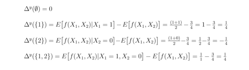
Second, we have to compute the prediction differences for all subsets of features, so we first compute the expected prediction if no feature values are known:
Now we can compute the prediction differences:
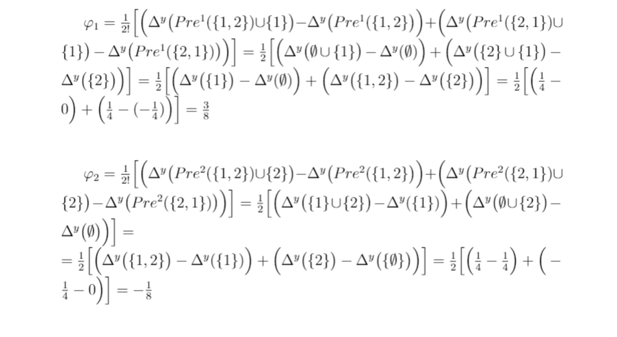
Finally, we can compute the contributions of the features:
The contribution of the first feature is positive while the contribution of the second feature is negative, which is reasonable. Since the class is 1 when at least one of the features is 1, the first feature of our instance made the model predict 1, so this value contributed to the model’s decision of predicting 1. On the contrary, the second feature made less probable that 1 was the predicted class, so it had a negative influence on the model’s decision. Additionally, the absolute value of the first contribution is larger than the second one, which means that the first feature was decisive for the prediction. Finally, note that the two contributions sum up to the initial difference between the prediction for this instance and the expected prediction when the feature values are unknown: φ₁+φ₂=3/8–1/8=1/4=1–3/4=f(1,0)-E[f(X₁,X₂)], which was assured by axiom 1.
In summary, the explanation produced by IME for the prediction of the instance (1,0) is that the model’s decision is influenced by both features, being the first feature more decisive in favor of (correctly) predicting class 1 than the second feature, whose value was against this decision.
This was a very simple example that we’ve been able to compute analytically, but these won’t be possible in real applications, in which we will need the approximated solution by the algorithm. In future posts I will explain how to explain predictions with Shapley Values using R and Python.
My blog is now on Medium ! Despite their high predictive performance, many machine learning techniques remain black boxes because it is difficult to understand the role of each feature and how it combines with others to produce a prediction. However, users need to understand and trust the decisions made by machine learning models, especially in sensitive fields such as medicine. For this reason, there is an increasing need of methods able to explain the individual predictions of a model, that is, a way to understand what features made the model give its prediction for a specific instance. A typical machine learning setting is shown in the following picture: Source: https://www.darpa.mil/program/explainable-artificial-intelligence We have a neural network (the machine learning model ) trained as an image classifier. This model would give a probability (let's say 0.98) that a cat appears in the picture (an observation ), so we could say that "our ...
My blog is now on Medium ! In a recent post I introduced three existing approaches to explain individual predictions of any machine learning model. In this post I will focus on one of them: Local Interpretable Model-agnostic Explanations ( LIME ), a method presented by Marco Tulio Ribeiro, Sameer Singh and Carlos Guestrin in 2016. In my opinion, its name perfectly summarizes the three basic ideas behind this explanation method: Model-agnosticism . In other words, model-independent, which means that LIME doesn’t make any assumptions about the model whose prediction is explained. It treats the model as a black-box, so the only way that it has to understand its behavior is perturbing the input and see how the predictions change. Interpretability . Explanations have to be easy to understand by users above all, which is not necessarily true for the feature space used by the model because it may use too many input variables (even a linear model can be difficult to interpret if it...
My blog is now on Medium ! A few months ago Google announced a new Google BigQuery feature called BigQuery ML, which is currently in Beta. It consists of a set of extensions of the SQL language that allows to create machine learning models, evaluate their predictive performance and make predictions for new data directly in BigQuery. Source: https://twitter.com/sfeir/status/1039135212633042945 One of the advantages of BigQuery ML (BQML) is that one only needs to know standard SQL in order to use it (without needing to use R or Python to train models), which makes machine learning more accessible. It even handles data transformation, training/test sets split, etc. In addition, it reduces the training time of models because it works directly where the data is stored (BigQuery) and, consequently, it is not necessary to export the data to other tools. But not everything is an advantage. First of all, the implemented models are currently limited (although we will see that...


Comments
Post a Comment